MATLAB Dual-Polarimetric Radar Project

For my METR 4330 project, I used MATLAB to develop a program that will create a plot of average reflectivity versus differential reflectivity. In dual-polarimetric radar, differential reflectivity (ZDR) is the common logarithm of the ratio of horizontal reflectivity to vertical reflectivity. This term can be very useful in determining the shape of the radar target, and thus, the type of hydrometeor. Spherical objects will have a differential reflectivity value of close to 0 (ratio of 1, then the log of 1 is 0). Spherical objects tend to be either small rain drops, hail, graupel, or snow. The combination of reflectivity and differential reflectivity can help us determine what hydrometeor is likely being seen by the radar. For example, a radar bin with high reflectivity and low differential reflectivity (large spherical object) is likely hail whereas a bin with low reflectivity and low differential reflectivity (small spherical object) is likely snow or small rain drops. Differential reflectivity is most useful for hail detection. The other dual-polarimetric variable used in this project was correlation coefficient. Correlation coefficient (CC) indicates how similar all targets in a radar bin are to each other, meaning a CC near 1 would indicate that almost all objects in the radar bin are the same size and shape whereas lower values would indicate a mix of objects with very low values indicating ground clutter. Below are a set of radar images used in this case study.

KOUN Base Reflectivity

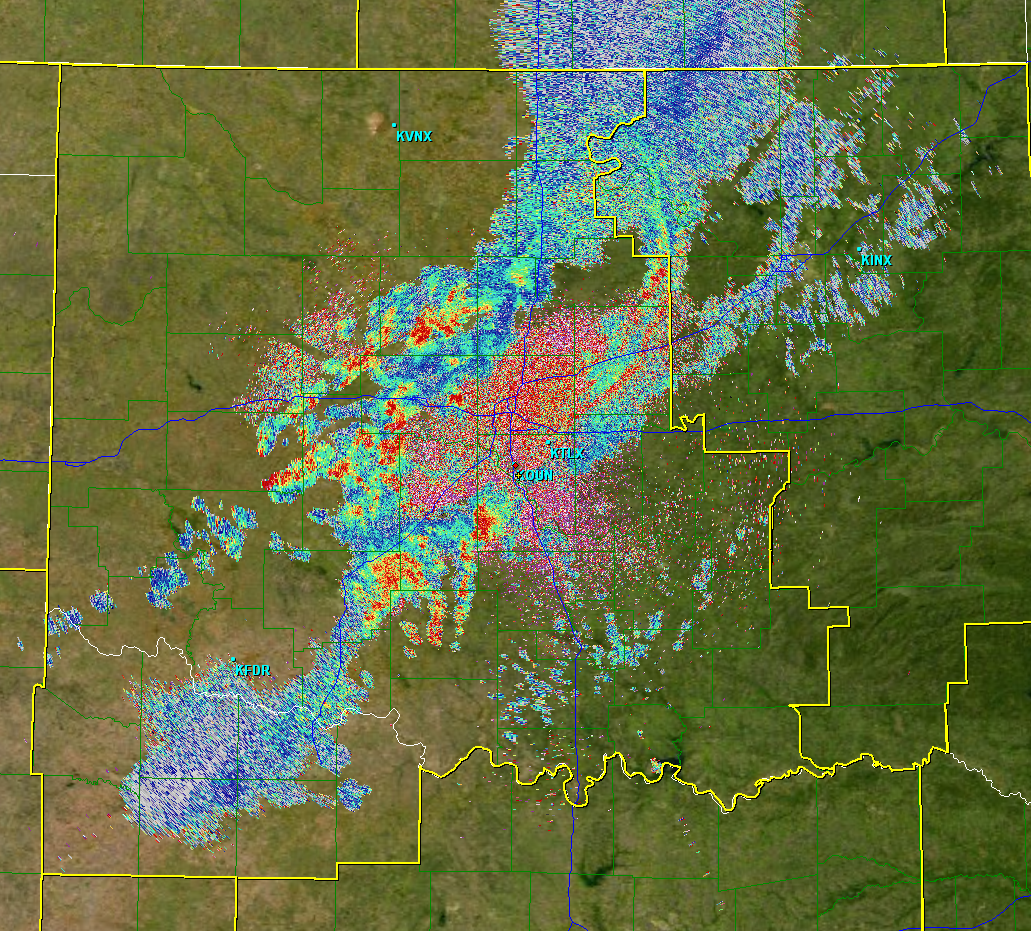
KOUN Differential Reflectivity

KOUN Correlation Coefficient

The program I wrote serves two purposes: (1) exploring the expected values of ZDR for a given value of Z, and (2) determining the calibration of the ZDR by testing it against known values.

The first portion of the program is where the user enters their initial values:

mindistance: This is the minimum distance the user wishes to examine from the radar site. Generally, a user would want to start at least 25 km from the radar since there tends to be a high amount of ground clutter close to the radar site.
maxdistance: This is the maximum distance the user wishes to examine from the radar site.
elevationcut: This is the elevation scan the user wishes to use.
lowerz: This is the minimum reflectivity to check the average ZDR against.
upperz: This is the maximum reflectivity to check the average ZDR against.
rhomin: This is the minimum correlation coefficient to use. By setting a high correlation coefficient, this ensures the user that the bins being used in the analysis are only bins containing mostly precipitation and not ground clutter. In otherwords, we set this high if we only want to look at the weather.

The second portion of the program checks the input for user errors. The volume coverage pattern (VCP) is used to determine the number of cuts. This checks to make sure the user input a valid cut number. For example, in VCP 32, the user can only enter a cut number (elevationcut) of only up to 8. The minimum distance is checked first. If the user enters a minimum distance that is either less than 1 km or is greater than the maximum distance, the minimum distance is reset to 1 km. A similar check is used for maximum distance. The elevationcut is checked by making sure the user enters a value of at least 1 and not a value that exceeds the number of available cuts for the given VCP mode. If the number input by the user is invalid, the elevationcut defaults to 1, the lowest cut. The lowerz is not permitted to be below -15 dBZ and the upperz is not permitted to be above 80 dBZ. The final check makes sure the CC is not set over 1 (the theoretical maximum for CC).

The third portion of the program creates a mask based on the user's inputs for lowerz, upperz, and rhomin. This mask sets all Z and ZDR values not in the input reflectivity range and below the CC limit to not-a-number (NaN).

The fourth portion of the program computes the ZDR average for each value of reflectivity. This takes all bins for a particular reflectivity value and determines the average of the differential reflectivity of all corresponding bins.

The final portion of the program generates a plot with reflectivity values on the x-axis and differential reflectivity values on the y-axis. The green dots that are plotted indicate the individual differential reflectivity values. The red line that is plotted indicates the average ZDR value for a given Z value. The average ZDR for the entire range of reflectivities is plotted as text towards the top of the plot.

Click image to enlarge it.

The plot above shows the expected trend of ZDR with respect to Z. As the reflectivities increase the differential reflectivity values also increase. This is because the larger droplets tend to be more oblate, thus resulting in higher differential reflectivity values (larger horizontal reflectivity and vertical reflectivity). In this particular data case, there were a few storms that produced small hail, thus the few low values of ZDR in the higher Z values, but the majority of the returns during this data case were from rain drops of varying size.