Application of the Quasi-Inverse Method for Data Assimilation

Seon Ki Park^1,* and Eugenia Kalnay<sup>1,2,3,*


1</sup>Cooperative Institute for Mesoscale Meteorological Studies
²School of Meteorology
University of Oklahoma, Norman, OK 73019, U.S.A.

³National Center for Environmental Prediction
NWS/NOAA, Washington, D.C., 20233, U.S.A.

^*Current affiliation: Department of Meteorology, University of Maryland, College Park, MD 20742, U.S.A.

1. Introduction

Using a theoretical relationship (i.e., physical laws), for given values of model parameters, a `direct' (or forward) problem aims at predicting the values of some observable quantities. In contrast, for given measurements of observable quantities, an `inverse' problem aims at obtaining the values of model parameters (Tarantola 1987).

Over the past two decades, many inverse problems in meteorology have been solved using the adjoint models of corresponding meteorological prediction systems. These include the generation of singular vectors for ensemble prediction (e.g., Molteni et al. 1996); four-dimensional variational data assimilation (e.g., Lewis and Derber 1985; Le Dimet and Talagrand 1986; Courtier et al. 1994); forecast sensitivity to the initial conditions (Rabier et al. 1996; Pu et al. 1997a); and targeted observations (e.g., Rohaly et al. 1998; Pu et al. 1998).

The four-dimensional variational data assimilation (4D-Var) using the adjoint model, in which a cost function (weighted squared distance between model solutions and observations) is minimized via iterative processes, is considered as the most promising tool for fitting model solutions to observations and has received considerable attention in recent years (Derber 1989; Courtier et al. 1994; Zupanski 1993; and many other papers). However, a major problems with the adjoint 4D-Var is that it takes a large computational cost to obtain an optimal initial condition because several hundreds iterations are often required for the minimizations process to converge. Thus implementing the complete adjoint 4D-Var scheme into the operational system is practically infeasible. For example, ECMWF has the most powerful supercomputer available but still has implemented a 4D-Var package into its operational system with only a simplified version (Bouttier and Rabier 1997). In addition, the assimilation period affects the quality of data assimilation results. An inadequately long assimilation period may lead to a cost function which has multiple minima and thus convergence to a local minium (Li 1991). An inadequately short period may not allow the information of assimilated data to propagate to the whole model domain (Luong et al. 1998).

When applied to a stormscale prediction model, whose intrinsic predictability limit extends to only a few hours, the time required for data assimilation becomes more restrictive. From our experiences with the operational testing of a stormscale model, the Advanced Regional Prediction System (ARPS; Xue et al. 1995), the model outputs for the 7-hr forecast are available about after 3 hrs without the 4D-Var process (e.g., Droegemeier et al. 1996). When the 4D-Var is included additional computing times are required, which results in a shorter lead time. Thus the data assimilation process needs to be finished in a short time. Although the assimilation period can be set to be very short, e.g., a few minutes (Wang et al. 1997; Park and Droegemeier 1997a), the obtained optimal initial conditions do not necessarily produce optimal forecast for a forecast time longer than the assimilation period because the stormscale models include many strongly nonlinear microphysical processes. In addition, the information from the assimilated data might not be able to propagate to the whole model domain within such a short assimilation period (Luong et al. 1998). Furthermore, the linear adjoint model involves errors in describing correct gradient information of the original nonlinear forecast model and those errors can be serious for stormscale models in which strongly nonlinear and discontinuous microphysical processes are included (see Park and Droegemeier 1997b).

Recently Wang et al. (1997) suggested the use of inverse model integrations in order to accelerate the convergence of 4D-Var. They developed a new optimization method called adjoint Newton algorithm (ANA) and demonstrated the efficiency of the ANA when applied to a simplified 4D-Var problem using ARPS. In the ANA, the Newton descent direction is obtained by a backward integration of the tangent linear model (TLM), in which the sign of timestep is changed (i.e., inverse). Here, the sign of dissipative terms is also changed in order to avoid computational blow-up (i.e., quasi-inverse). By adopting this ``quasi-inverse'' approach and assuming the availability of a complete set of observations at final time, Wang et al. (1997) showed that the ANA converged in an order of magnitude fewer iterations, and to an error level an order of magnitude smaller than the conventional adjoint approach to solve the same (simplified) 4D-Var problem. However, their application of the quasi-inverse method was limited to finding the Newton descent direction only, and a complete data set at the end of the assimilation period.

The quasi-inverse technique can be applied to either the tangent linear or the full nonlinear model, each of which has advantages for different applications. Pu et al. (1997) showed that for the problem of forecast sensitivity, closely related to 4D-Var, a backward integration with the quasi-inverse TLM (Q-ILM) gave results far superior to those obtained using the adjoint model. The Q-ILM has been tested successfully at NCEP in several different applications, e.g., forecast error sensitivity analysis and data assimilation (Pu et al. 1997), and adaptive observations (Pu et al. 1998). Kalnay and Pu (1998) suggested the use of Q-ILM in a more general way in data assimilation problems. Kalnay et al. (1999) demonstrated, using the Q-ILMs of simple models, a much faster performance of the quasi-inverse method in data assimilation than the conventional adjoint 4D-Var method. The former is dubbed ``inverse 3D-Var'' (I3D-Var) in the sense that the observation is used only once at the end of the assimilation interval.

While the I3D-Var does not require to run either the adjoint model or the minimization process, the adjoint 4D-Var requires to run both the adjoint model, to provide the gradient information to the minimization algorithm, and the minimization process. For the minimization of a quadratic function such as the cost function in the 4D-Var, the full-Newton method is the most ideal algorithm because it brings to the minimum of cost function in just a single iteration. However, it has never been used in a realistic large-scale optimization problems because the computation and storage of the Hessian and its inverse are too costly to be practical (Gill 1981).

There exist several methods for large-scale unconstrained optimization such as quasi-Newton (Gill and Murray 1972), limited-memory quasi-Newton (LBFGS - Liu and Nocedal 1989), truncated Newton (Nash 1984), adjoint truncated-Newton (Wang et al. 1995), adjoint Newton (Wang et al. 1997, 1998), and conjugate gradients methods (Navon and Legler 1987). When applied to meteorological 4D-Var problems, these algorithms mostly require a few tens to hundereds iterations to reach a local minimum of cost function. Reviews on various optimization algorithms are given in some texbooks, e.g., Gill (1981), Tarantola (1987), and Polak (1997). In the following, we provide a brief overview on the theoretical background of the I3D-Var. For a more detailed discussion see Kalnay et al. (1999).

2. Formulation of I3D-Var

The major goal of I3D-Var is to find an increment in initial conditions ${{\delta}x}$ that ``optimally'' corrects a perceived forecast error at the final time t. Here, the cost function includes both data and background distances. In order to maintain the ability to solve the minimization efficiently, however, the background term is estimated at the end of the interval, rather than at the beginning as in Lorenc (1986).

Assume (for the moment) that data y^o is available at the end of the assimilation interval t, with ${{\delta}x}$=x^a-x^b, ${{\delta}y}$=y^o-$\mathsf{H}$(x^b). Here x^a and x^b are the analysis and first guess, respectively, and $\mathsf{H}$is the ``forward observation operator'' which converts the model first guess into first guess observations (see Ide et al. 1997 for notation). The cost function that we minimize is the 3D-Var cost function at the end of the interval. It is given by the distance to the background of the forecast at the end of the time interval (weighted by the inverse of the forecast error covariance B), plus the distance to the observations (weighted by the inverse of the observational error covariance R), also at the end of the interval:

$$J = \frac{1}{2}(L{{\delta}x})^{T}B^{-1}(L{{\delta}x}) + \fra... ...L{{\delta}x}-{{\delta}y}]^{T}R^{-1}[HL{{\delta}x}-{{\delta}y}].$$ (1)

Here ${{\delta}x}$ (the control variable) is the difference between the analysis and the background (at the present iteration) at the beginning of the assimilation window, L and L^Tare the TLM and its adjoint, respectively, and H is the tangent linear version of the forward observation operator $\mathsf{H}$. If we take the gradient of J with respect to the initial change ${{\delta}x}$,we obtain

$${{\nabla}J} = L^{T}\{B^{-1}L{{\delta}x} + H^{T}R^{-1}[HL{{\delta}x}-{{\delta}y}]\}.$$ (2)

From this equation we see that the gradient of the cost function is given by the backward adjoint integration of the rhs terms in (2). In the adjoint 4D-Var, an iterative algorithm (such as quasi-Newton, conjugate gradient, or steepest descent) is used to estimate an optimum perturbation:

$${{\delta}x}^{i}={\alpha}_{i}{{\nabla}J}^{i-1}$$ (3)

and the procedure is repeated until after many iterations ${{\nabla}J}$becomes very small, and the minimum of J is reached. It should be noted that in order to determine an optimal value for the step size ${\alpha}_{i}$, the minimization algorithms such as conjugate gradient or quasi-Newton require additional computations of the gradient ${{\nabla}J}^{i-1}$, so that the number of direct and adjoint integrations required by the 4D-Var can be significantly larger than the number of iterations.

In the I3D-Var, however, we seek to obtain directly the ``perfect solution'' i.e., the ${{\delta}x}$ that makes ${{\nabla}J}$=0 for small ${{\delta}x}$. From (2) we can eliminate the adjoint operator, and obtain the ``perfect'' solution given by

$$L{{\delta}x} = (B^{-1} + H^{T}R^{-1}H)^{-1}H^{T}R^{-1}{{\delta}y}.$$ (4)

Since we have a good approximation of L^-1 at hand (the quasi-inverse model obtained by integrating the tangent linear model backward, but changing the sign of frictional terms), we can apply it and obtain

$${{\delta}x} = L^{-1}(B^{-1} + H^{T}R^{-1}H)^{-1}H^{T}R^{-1}{{\delta}y}.$$ (5)

This can be interpreted as starting from the 3D-Var analysis increment at the end of the interval and integrating backwards with the TLM or an approximation of it. If we do not include the forecast error covariance term B^-1, (5) reduces to the ANA algorithm of Wang et al. (1997) except that we do not require line minimization. We have tested the I3D-VAR with the ARPS model and found that for this reason, the I3D-Var is computationally about twice as fast as Wang et al. (1997) ANA scheme.

Kalnay et al. (1999) proved that the I3D-Var is equivalent to solving the minimization problem (at each time level) using the full-Newton method. The results of Wang et al. (1997, 1998) and Pu et al. (1997) support considerable optimism for this method. For a quadratic function, the Newton algorithm (and the equivalent I3D-Var) converges in a single iteration. Since the cost functions used in the 4D-Var are close to quadratic functions, the I3D-Var can be considered equivalent to perfect preconditioning of the simplified 4D-Var problem.

3. Application to the Burgers' Equation

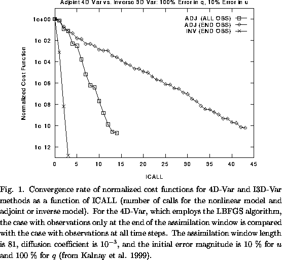
Figure 1 shows the performance of the I3D-Var and the 4D-Var (using LBFGS minimization algorithm) for a simple advection-diffusion problem (Burgers' equation) including a passive scalar transport, q. For an assimilation window of 81 time steps and errors of a 10% in initial velocity u and a 100% in q, using the I3D-Var in which observations are available only at the end of the interval, the cost function converges to 10^-13 of its original value after 3 iterations. However, the 4D-Var with data at the end of the interval requires 44 equivalent model integrations (both forward and adjoint) for the cost function to converge to 10^-10 of the original value. If we provide the 4D-Var with observations for every time step, the cost function converges to the same order in 12 time integrations.

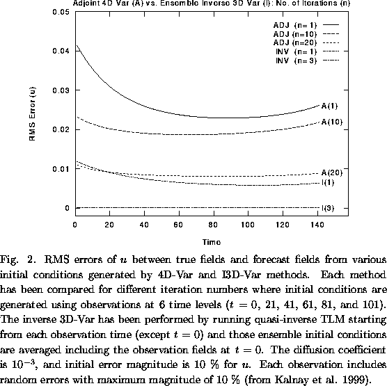
If there are data at different time levels we can choose to bring the data increments to the same initial time level so that the increments corresponding to the different data can be averaged, with weights that may depend on the time level or the type of data. For applications in which ``knowing the future'' is allowed, such as reanalysis, the observational increments could be brought to the center of an interval, and used for the final analysis.

Figure 2 shows preliminary results of having multiple time levels in the observations using the Burgers' equation. Random errors are included in observations with a maximum amplitude of 10% of the total range. The observational increments from different observational times are brought backwards to the same initial time level, at which those increments are averaged to yield the averaged initial conditions. Then forecasts beyond the assimilation period (101 time steps) up to 141 time steps are compared for initial conditions obtained from the 4D-Var and those that are averaged from multiple (ensemble) I3D-Var. The results of the forecasts with one iteration of the I3D-Var were comparable to those of 20 iterations of the 4D-Var, whereas 3 iterations of the I3D-Var resulted in much better forecasts.

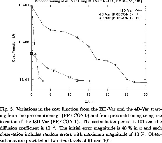
The I3D-Var also has some potential disadvantages. One of them is the growth of noise that projects on decaying modes during the backward integration (Kalnay et al. 1999). However, those errors decay again during the subsequent forward integration. We also found that the performance of I3D-Var is dependent upon the magnitude of dissipation. We believe that these problems can be overcome with further development and experimentation. At least the I3D-Var might serve as a preconditioner when carrying minimization in the framework of the 4D-Var. To test this idea, a preliminary experiment using the Burgers' equation is performed. In Fig. 3, using the initial conditions obtained from one iteration of the I3D-Var, the 4D-Var showed much better performance in minimizing the cost function. The result shows a possibility of using the I3D-Var as a preconditioner of the 4D-Var including full physics. The use of the I3D-Var may deal efficiently with the part of the spectrum of the Hessian of the cost function related to the dynamics part of the model. This will allow the minimization to focus only on the nonlinearities associated with the physics and result in a large computational economy (Navon, 1999; personal communication).

Some approaches similar to the I3D-Var, in the sense of the least squre fitting by solving the inverse matrix of the forward linear or nonlinear model operator, are also found in the inverse problems of other disciplines such as seismic waves (e.g., Gersztenkorn et al. 1986), electromagnetic data (e.g., Farquharson and Oldenburg 1998), and quantum dynamics (e.g., Caudill Jr. et al. 1994). For theoretical backgrounds on general inverse problems, see Tarantola (1989) and Anger (1993).

For a detailed discussion on the quasi-inverse method in the context of data assimilation and some results with simple models (Burgers' equation and Lorenz model), see Kalnay et al. (1999) and its web page at ``http://weather.ou.edu/~ekalnay/INV3DVARpap/kal_web1_rev/''.

References

Anger, G., 1993: Basic principles of inverse problems. Inverse Problems: Principles and Applications in Geophysics, Technology, and Medicine, G. Anger, R. Gorenflo, H. Jochmann, H. Moritz, and W. Webers, Eds., Akademie Verlag, 24-36.

Bouttier, F., and F. Rabier, 1997: The operational implementation of 4D-Var. ECMWF Newsletter, No. 78, 2-5.

Courtier, P., J.-N. Thepaut, and A. Hollingsworth, 1994: A strategy for operational implementation of 4D-Var using an incremental approach. Quart. J. Roy. Met. Soc., 120, 1367-1388.

Caudil Jr., L. F., H. Rabitz, and A. Askar, 1994: A direct method for the inversion of physical systems. Inverse Problems, 10, 1099-1114.

Derber, J. C., 1989: A variational continuous assimilation technique. Mon. Wea. Rev., 117, 2437-2446.

Droegemeier, K. K., M. Xue, K. Brewster, Y. Liu, S. K. Park, F. H. Carr, J. Mewes, J. Zong, A. Sathye, G. Basset, M. Zou, R. Carpenter, D. McCarthy, D. Andra, P. Janish, R. Graham, S. Sanielvici, J. Brown, B. Loftis, and K. McLain, 1996: The 1996 CAPS operational forecasting period: Realtime storm-scale NWP, Part I: Goals and methodology. Preprints, 11th Conf. on Numerical Weather Prediction, August 19-23, Norfolk, VA, Amer. Meteor. Soc., 294-296.

Farquharson, C. G., and D. W. Oldenburg, 1998: Non-linear inversion using general measures of data misfit and model structure. Geophys. J. Int., 134, 213-227.

Gersztenkorn, A., J. B. Bednar, and L. R. Lines, 1986: Robust iterative inversion for the one-dimensional acoustic wave equation. Geophysics, 51, 357-368.

Gill, P. E., and W. Murray, 1972: Quasi-Newton methods for unconstrained optimization. J. Inds. Maths Appl., 9, 91-108.

Gill, P. E., W. Murray and M. H. Wright, 1981: Practical Optimization. Academic Press, pp 401.

Ide, K., P. Courtier, M. Ghil and A. Lorenc, 1997: Unified notation for data assimilation: operational, sequential and variational. J. of Meteor. Soc. Japan, 75 (1B), pp 181-197.

Kalnay, E., and Z.-X. Pu, 1998: Application of the quasi-inverse method to accelerate 4D-Var. Preprints, 12th Conf. on Numerical Weather Prediction, Phoenix, AZ, Amer. Meteor. Soc., 41-42.

Kalnay, E., S. K. Park, Z.-X. Pu, and J. Gao, 1999: Application of the quasi-inverse method to data assimilation. Mon. Wea. Rev., Accepted for publication.

Le Dimet, F. X., and O. Talagrand, 1986: Variational algorithms for analysis and assimilation of meteorological observation: Theoretical aspects. Tellus, 38A, 97-110.

Lewis, J. M., and J. C. Derber, 1985: The use of adjoint equations to solve a variational adjustment problem with convective constraints. Tellus, 37A, 309-322.

Li, Y., 1991: A note on the uniqueness problem of variational adjustment approach to four-dimensional data assimilation. J. Meteor. Soc. Japan, 69, 581-585.

Liu, D. C. and J. Nocedal, 1989: On the limited memory BFGS method for large scale minimization. Math. Prog., 45, 503-528.

Lorenc, A. C., 1986: Analysis methods for numerical weather prediction. Quart. J. Roy. Meteor. Soc., 112, 1177-1194.

Luong, B., J. Blum, and J. Verron, 1998: A variational method for the resolution of a data assimilation problem in oceanography. Inverse Problems, 14, 979-997.

Nash, S. G., 1984: Truncated-Newton methods for large-scale function minimization. Applications of Nonlinear Programming to Optimization and Control, H. E. Rauch, Ed., Pergamon Press, 91-100.

Navon, I. M., and D. M. Legler, 1987: Conjugate-gradient methods for large-scale minimization in meteorology. Mon. Wea. Rev., 115, 1479-1502.

Molteni, F., R. Buizza, T. N. Palmer, and T. Petroliagis, 1996: The ECMWF Ensemble Prediction System: Methodology and validation. Quart. J. Roy. Meteor. Soc., 122, 73-119.

Park, S. K., 1999: Predictability of convective rainfall associated with nonlinearity for water vapor perturbations in a numerically-simulated storm. Submitted to J. Geophys. Res.

Park, S. K., and K. K. Droegemeier, 1997a: 4DVAR with a moist adjoint applied to deep convective storms - Simulated data experiments. Preprints, 2nd US-Korea Joint Workshop for Storm- and Mesoscale Weather Analysis and Prediction, October 7-10, Seoul, Korea, 52-56.

Park, S. K., and K. K. Droegemeier, 1997b: Validity of the tangent linear approximation in a moist convective cloud model. Mon. Wea. Rev., 125, 3320-3340.

Polak, E., 1997: Optimization: Alogorithms and consistent approximations. Springer-Verlag, 779 pp.

Pu, Z.-X., E. Kalnay, J. Sela, and I. Szunyogh, 1997: Sensitivity of forecast errors to initial conditions with a quasi-inverse linear model. Mon. Wea. Rev., 125, 2479-2503.

Pu, Z.-X., S. J. Lord and E. Kalnay, 1998: Forecast Sensitivity with dropwindsonde data and targeted observations. Tellus, 50A, 391-410.

Rabier, F., E. Klinker, P. Courtier and A. Hollingsworth, 1996: Sensitivity of forecast errors to initial conditions. Quart. J. Roy. Meteor. Soc., 122, 121-150.

Reynolds, C. A., T. N. Palmer, 1998: Decaying singular vectors and their impact on analysis and forecast correction. J. Atmos. Sci., 55, 3005-3023.

Rohaly, G. D., R. H. Langland, and R. Gelaro, 1998: Identifying regions where the forecast of tropical cyclone tracks is most sensitive to initial condition uncertainty using adjoint methods. Preprints, 12th Conf. on Numerical Weather Prediction, Phoenix, AZ, Amer. Meteor. Soc., 337-340.

Sneider, R., 1998: The role of nonlinearity in inverse problems. Inverse Problems, 14, 387-404.

Tarantola, A., 1987: Inverse Problem Theory. Elsevier Science, 613 pp.

Wang, Z., I. M. Navon, X. Zou, and F. X. Le Dimet, 1995: A truncated Newton optimization algorithm in meteorology applications with analytic Hessian/vector products. Comput. Optimization Appl., 4, 241-262.

Wang, Z., K. K. Droegemeier, L. White and I. M. Navon, 1997: Application of a new adjoint Newton algorithm to the 3D ARPS storm-scale model using simulated data. Mon. Wea. Rev., 125, 2460-2478.

Wang, Z., K. K. Droegemeier, and L. White, 1998: The adjoint Newton algorithm for large-scale unconstrained optimization in meteorology applications. Comput. Optimization Appl., 10, 283-320.

Xue, M., K. K. Droegemeier, V. Wong, A. Shapiro, and K. Brewster, 1995: ARPS Version 4.0 Users' Guide. Center for Analysis and Prediction of Storms, University of Oklahoma, 380 pp. [Available from Center for Analysis and Prediction of Storms, University of Oklahoma, Norman, OK, 73019.]

Zupanski, M., 1993: Regional 4-dimensional variational data assimilation in a quasi-opera- tional forecasting environment. Mon. Wea. Rev., 121, 2396-2408.