5.B6

SENSITIVITY OF 3-D CONVECTIVE STORM EVOLUTION TO WATER VAPOR AND IMPLICATIONS FOR VARIATIONAL DATA ASSIMILATION

Seon Ki Park and Kelvin K. Droegemeier
Center for Analysis and Prediction of Storms and School of Meteorology
University of Oklahoma, Norman, OK 73019

1. INTRODUCTION

Model parameters, both physical and computational, as well as initial and boundary conditions are essential factors in controlling the dynamical evolution of flows in atmospheric numerical models. For deep convective storms, their effects have been evaluated through the deterministic approach of sensitivity analysis (Park 1996), which employs a set of differential equations such as the tangent linear model (TLM) and the adjoint model (ADJM). Here, the sensitivity is defined as the gradient of the model response or output with respect to any input parameter.

Although having been used substantially for both sensitivity analysis and variational data assimilation in meteorology, the ADJM, especially of 3-D models, is still routinely generated by hand. The gradients can be computed efficiently and accurately by using automatic differentiation (AD) tools, which apply the chain rule systematically to elementary operations or functions to generate derivative codes of given nonlinear models. In this study, we apply a general purpose AD tool called ADIFOR (Automatic DIfferentiation of FORtran; Bischof et al. 1992) to the 3-D Advanced Regional Prediction System (ARPS; Xue et al. 1995) to generate a sensitivity-enhanced code (SE-ARPS) capable of providing derivatives of all model output variables and related diagnostic (derived) parameters (i.e., dependent variables; DV) as a function of specified control parameters, including initial and boundary conditions as well as physical and computational constants (i.e., independent variables; IV).

Given the strong influence that water vapor has on atmospheric processes, particularly convective storms, we compute the sensitivity of model outputs with respect to water vapor. We also compute sensitivities of the cost function, which measures distance in the Euclidean norm between the observations and model results, with respect to all model variables. Subsequently, we discuss implications of the sensitivity results to data assimilation.

2. SENSITIVITY TO PERTURBATIONS

In 3-D models, the number of IVs is potentially very large when grid variables are considered, and this may inhibit the practical computation of sensitivity because of memory limitations. Although data assimilation requires the gradient of a cost function with respect to specified control parameters, we may need, in many forecasting problems, the sensitivities of model responses to perturbations only in specific regions. By introducing an artificial perturbation parameter, e, into ARPS, we let ADIFOR generate a sensitivity code that regards e as one of the IVs (Bischof et al. 1995).

For example, suppose the water vapor field, , is perturbed by a factor e. Then any quantity P that is influenced by implicitly depends upon e. Expanding P(e) in a Taylor series about the reference state [P(e = 0)] and retaining only the first-order term, we obtain an approximation to the sensitivity of P with respect to e:

Here, can be interpreted as the sensitivity of P to a uniform fractional change in . Accordingly, the relative sensitivity coefficient (RSC) is defined as normalized by its nonlinear counterparts (P/e) and describes the percentage change in P due to a 1 % perturbation (e) in (Park 1996).

Since the perturbation e is added to the input parameters, which already have their own characteristic distribution in the model domain, sensitivities computed from this approach implicitly involve the characteristics of those parameters. We limit our experiments only to at initial and intermediate times excluding boundary conditions.

3. MODEL, CONTROL SIMULATION AND TLM VALIDATION

We employ the full-physics ARPS (version 4.0), which is three dimensional, fully compressible, and nonhydrostatic. The prognostic variables, solved on the Arakawa C grid include Cartesian velocity components (u, v and w), perturbations of potential temperature ( ) and pressure (p), mixing ratios of water vapor ( ), cloud water ( ) and rain water ( ), and turbulent kinetic energy. An extensive description of the model can be found in the ARPS user's guide (Xue et al. 1995).

The computational domain consists of grids in the horizontal with a grid size of 1 km. In the vertical, a stretched grid system is employed with 35 levels and a resolution of 150 m near the ground and 850 m at the top. The model is run for 140 min, with a large timestep of 6 sec and a small timestep of 1 sec. The detailed model configuration for our experiments is described in Park (1996).

The simulation is made using the supercell HALF4 hodograph and thermodynamic sounding from Droegemeier et al. (1993). The simulated supercell develops rapidly during the first 30 minutes and becomes quasi-steady thereafter, with a sustained updraft of around 47 m/s. Major storm features including the surface outflow boundary (dotted lines) are shown in Figure 1. The isolated supercell storm becomes dominant after 60 min and travels southeastward along the leading edge of the expanding cold pool. A secondary storm develops northeast of the main storm after 100 min, merging into the main storm by 140 min.

Figure 1: Control simulation: w at 4.0 km (positive in solid and negative in dashed lines at the interval of 4.0 m s

) and perturbation

at surface (dotted lines with contours larger than -2.0 K at the interval of 0.5 K) at a) 50 min and b) 90 min.

Since the sensitivity equation is based on the tangent linear approximation, the accuracy of sensitivity results highly depends on the validity of TLM. For a 1 % perturbation in the initial

field, the TLM results produced by the SE-ARPS describe the nonlinear perturbation fields very accurately up to 50 min. For a 10 % perturbation, which is typical for observational errors of

in the lower troposphere, the TLM is valid for about 30 min. Considering the highly nonlinear and discontinuous properties of solutions in the moist convective model, the results are very encouraging for studies of storm predictability, variational data assimilation, Doppler radar retrieval, and ensemble forecasting. A detailed discussion of the validity of the TLM is provided in Park (1996).

4. RESULTS AND DISCUSSION

We investigate the effect of perturbations in within four different regions of the environment: ( ) inside the rain region above cloud base, ( ) in the ambient environment outside the rain region and above cloud base, ( ) the updraft region (including w = 0) in the subcloud layer, and ( ) the downdraft region in the subcloud layer.

We run the SE-ARPS starting at 90 min, when the supercell storm is fully mature (see Figure 1b). The cloud base at 90 min is around 485 m. Three model levels are involved in the subcloud layer. The numbers of grid points involved in perturbation are 8280 for , 61720 for , 5972 for , and 4028 for . Among the many available results, we discuss the sensitivity of vertical velocity (w), which is an important parameter describing storm intensity.

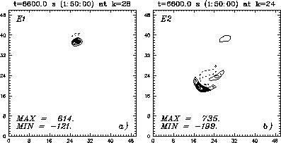
Figure 2 shows the domain maximum sensitivity of w at 110 min with respect to perturbations and at 90 min. At 110 min, in the control simulation, the main updraft is located near the center of the domain with a lima-bean shape, while a prominent secondary storm exists to the northeast. The sensitivities to perturbations below cloud base (i.e., and ) are much smaller than those above cloud base (i.e., and ). The location of the largest sensitivity differs for different perturbations. The largest w sensitivity to the perturbation occurs in the secondary storm near the cloud top, while that to the perturbation stays in the main storm at lower levels. The maximum sensitivity value of 614 in Figure 2a implies a change of w by 6.14 m s due to a 1 % perturbation ( ) in . For perturbations and , the largest sensitivity is observed at both the main and secondary storms (not shown).

Figure 2: Domain maximum sensitivity of w at t = 110 min with respect to the

perturbations of a)

and b)

at t = 90 min (at the interval of 100 m s

When moisture perturbations are added inside the cloud, they are advected out rapidly due to strong updraft and go into the environment, where they change it and thus influence secondary storms. When moisture is increased by the same factor outside the cloud, the amount of perturbation added is small because the moisture in the ambient air is small; thus, such perturbations might not be sufficient to affect the secondary storm. However, they can affect the main storm through mechanisms involving turbulent mixing and entrainment.

We now discuss the sensitivity results in the cost function and their implications on data assimilation. The cost function, J, is defined as the squared distance between the model states, , and the corresponding observations, :

where denotes a scalar product between and and n represents the time index. is a weighting factor matrix as defined in Park (1996). Applying this factor, the cost function is nondimensionalized and normalized at the beginning of the variational data assimilation window. Sensitivities of J are computed for perturbations in all model variables both inside and outside the rain region of the storm.

We consider the control simulation as our pseudo-observations. The sensitivity period is 30 min, from t = 80 min to t = 110 min. A 1 % perturbation is added to all variables at all grid points at 80 min for the perturbation run, which serves as the nonlinear basic field for the sensitivity computation. With this perturbation, model solutions show little difference from the pseudo-observations.

For perturbations inside the rain region, the largest sensitivity in the cost function (i.e., forecasting error) is due to variablity in , followed by p and . Among the moisture variables inside the cloud, exerts the largest influence on J, followed by and . Perturbations in the momentum variables (u, v and w) inside the rain region yield small changes in J. The sensitivities are generally smaller for perturbations outside the rain region. The largest sensitivity is due to , followed by and p. Since and are effectively zero in the ambient air, the sensitivities of J to them are extremely small.

Figure 3 depicts the RSC of J with respect to and p inside the rain region. The p field has the largest effect on J during the early sensitivity period. This is because p is directly responsible for the mass balance through pressure gradient forces in the momentum equations. When p is perturbed, the flow accelerates until terms involving the velocity become comparable with the pressure gradient force. Therefore, the flow immediately and significantly responds to the p perturbations. In contrast, perturbations in affect the system initially through only the buoyancy term in the vertical momentum equation, and then other variables through mass continuity. Hence, during the early sensitivity period, the p perturbations exert the largest influence on forecast errors among all variables. However, the increased buoyancy through the perturbation eventually influences storm dynamics and forecast error.

Figure 3: Relative sensitivities of cost function with respect to perturbations in

(white circle) and p (black circle) inside the cloud at t = 80 min.

When applied to variational data assimilation, sensitivity information, especially derivatives of the cost function with respect to all initial fields, can indicate which initial field must be modified by a large amount and which may be altered by only a small amount to change the cost function on the way to its minimum state. With this information, the minimization algorithm can be appled in a selective way to save computing time: that is, a variable that exerts little influence on the cost function may be put in the minimization process in a larger iteration step, while a variable with strong effect (e.g.,

) may be applied in every step. Our results indicate that the

perturbation has a greater impact on forecast error over a long time period than the p perturbation. Thus, we desire that our initial conditions have less error in temperature than pressure.

5. ACKNOWLEDGMENTS

This work was supported by the Center for Analysis and Prediction of Storms under Grant ATM91-20009 from the National Science Foundation (NSF) and by NSF Grant ATM92-22576 to the second author.

6. REFERENCES

Bischof, C., A. Carle, G. Corliss, A. Griewank, and P. Hovland, 1992: ADIFOR: Generating derivative codes from Fortran programs. Scientific Programming, 1, 11-29.

Bischof, C., G. Pusch, and R. Knoesel, 1995: Sensitivity analysis of the MM5 weather model using automatic differentiation. Preprint, MCS-P532-0895, Argonne National Laboratory, 14 pp.

Droegemeier, K.K., S.M. Lazarus, and R. Davies-Jones, 1993: The influence of helicity on numerically simulated convective storms. Mon. Wea. Rev., 121, 2005-2029.

Park, S.K., 1996: Sensitivity Analysis of Deep Convective Storms. Ph.D. thesis, School of Meteorology, University of Oklahoma, 245 pp.

Xue, M., K.K. Droegemeier, V. Wong, A. Shapiro, and K. Brewster, 1995: ARPS4.0 User's Guide. Center for Analysis and Prediction of Storms, University of Oklahoma, 380 pp.