The objective of this study is to find out the geographical areas to which the forecast aspect is the most sensitive. The gradients of J, i.e., the sensitivity patterns, are evaluated with respect to the model state variables.
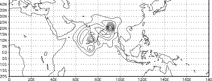
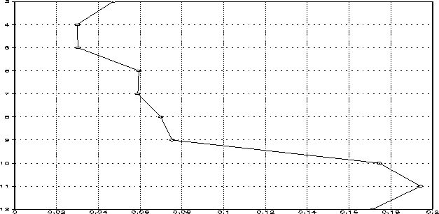
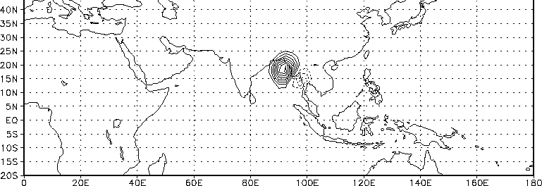
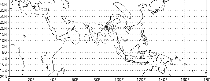
It is known that the analysis of moisture field is usually unreliable over the tropics due to the lack of sufficient observations, i.e., there is a large uncertainty in this analysis. Fig. 4 presents the squared sum of sensitivities with respect to the initial analysis of dewpoint depression for each model vertical level. The striking feature is that the forecast error is very sensitive to the initial analyses of dewpoint depression at the lowest three model vertical levels, while the sensitivities to the upper model levels are small. In order to provide a closer look at a single model vertical level, the sensitivity patterns with respect to the dewpoint depression at the lowest three model levels, i.e., model vertical levels 12, 11 and 10, are presented in Fig. 5 - Fig. 7, respectively. A large positive maximum center located at the upstream of the region with large forecast errors over the northern Bay was observed for both of the lowest two model levels, but a large negative maximum center was more pronounced at the third lowest level. The analyses of dewpoint depression at time t0 were diagnosed to be too dry over the northern Bay of Bengal at the lowest two model vertical levels. The results obtained also show that the model 1-day forecast error is most sensitive to the analysis errors in the dewpoint depression around 90E, 20N. Additional observations around this point are expected to improve the model 1-day forecast. The vertical cross-section at 20N for the sensitivity with respect to the dewpoint depression at time t0 is displayed in Fig. 8. The pattern is tilted in the vertical to the west, which indicates that further growth of the depression is sensitive to baroclinic perturbations at the initial time.
 |
 |
 |
 |
 |
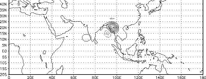
The sensitivity patterns with respect to the initial analysis of virtual temperature at model vertical levels 12 and 10 (Figures. 9 and 10) also indicate the locations of the geographical regions where the analysis problems lie in. The analyses of virtual temperature over the northern Bay of Bengal were diagnosed to be too low at model vertical level 12 and too high at model vertical level 10. The vertical cross-section at 20N is displayed in Fig. 11.
 |
 |
 |
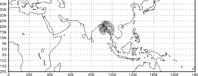
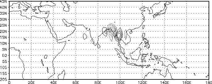
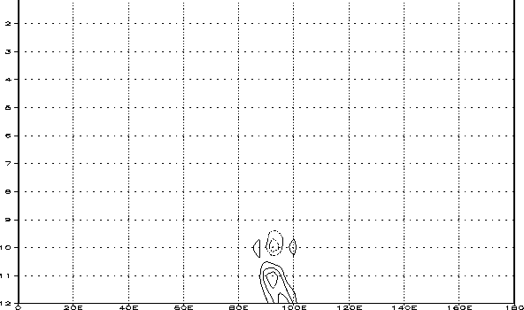
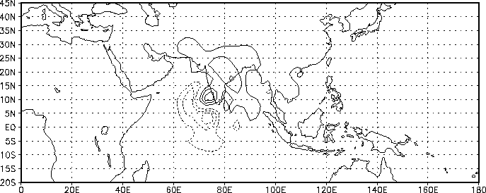
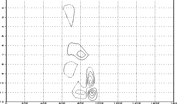
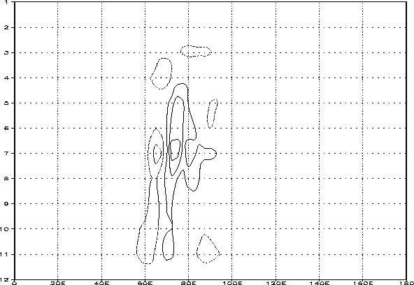
The calculation of the squared sum of sensitivities with respect to the initial analysis of vorticity for each model vertical level indicates that the model 1-day forecast error is sensitive to the uncertainties in the analysis at model vertical levels 11 and 7, which are approximately located above the surface and at 700 hPa, respectively. The sensitivity pattern with respect to the initial analyses of vorticity at model vertical levels 11 and 7 are displayed in Fig. 12 and Fig. 13, respectively. Two important areas with opposite signs are observed for both sensitivity patterns. The vertical cross-section at 20N for the sensitivity pattern with respect to vorticity at time t0 (Fig. 14) exhibited two large centers with opposite signs, both of which were located in the lower troposphere around 90E, 20N. This indicated that the forecast error was very sensitive to the vorticity analysis uncertainties in the lower atmosphere. One maximum center, which is located at model vertical level 7, was also observed in the vertical cross-section at 10N for the sensitivity pattern with respect to the initial analysis of vorticity (Fig. 15), and a westward-tilting of the vertical structure was not observed. The analysis uncertainties at model vertical level 7 are mainly distributed over the eastern Arabian Sea, while the analysis uncertainties at model vertical level 11 are mainly located around 90E, 20N.
 |
 |
 |
 |
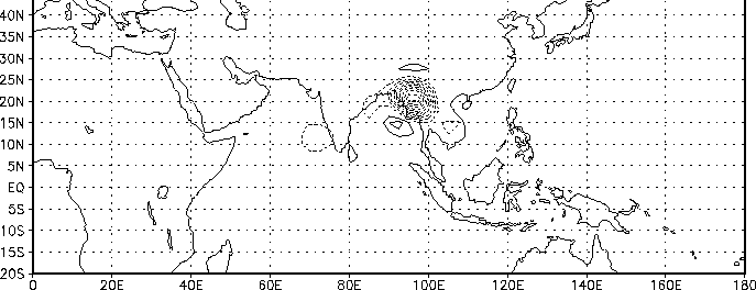
The sensitivity signal was also calculated in order to pinpoint the overall locations of the analysis uncertainties. It is represented by the sum of squares of the sensitivity patterns throughout the whole range of vertical levels. The sensitivity signals for vorticity and dewpoint depression are displayed in Figures 16 and 17, respectively. It is apparent that the model 1-day forecast error is most sensitive to the analysis errors located at around 90E, 20N over the northern Bay of Bengal.