Steven M. Cavallo

Real-time images and animations

Arctic sea ice forecasts Ensemble forecast of upcoming minimum sea ice extent
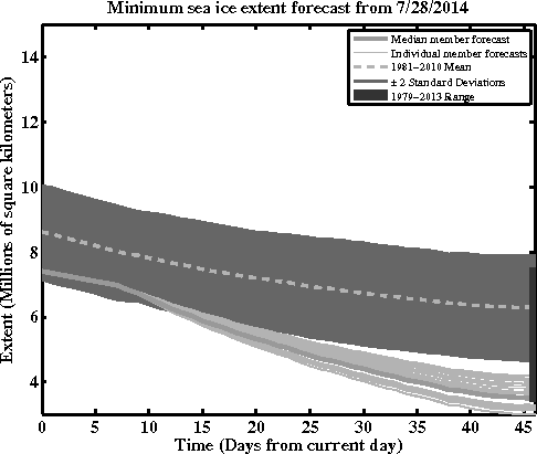
Minimum sea ice extent forecasts showing individual ensemble members (solid, light gray) and the ensemble median (solid, dark gray). The 1981-2010 climatology is shown for comparison (light, dashed gray) along with the +/- 2 standard deviation range (dark gray shading). The dark gray vertical bar on the last time denotes the range of minimum sea extent observed from 1979-2012. Ensemble forecasts are computed from a stochastic model by Steven Cavallo using past observations combined with the most recent estimates of the atmospheric state using NCEP/NCAR reanalysis data. Loop of this year's forecasts Loop of previous year's forecasts
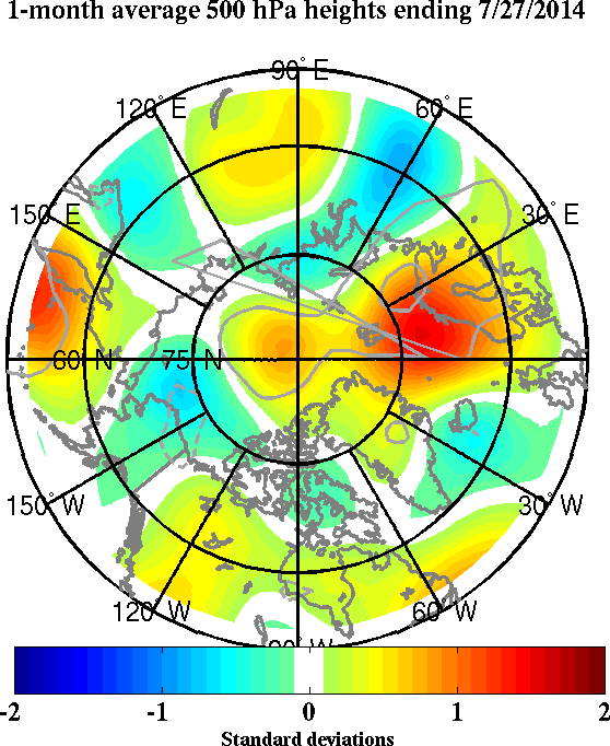
500 hPa height loop and latest image Colors show the standardized anomalies of 500 hPa geopotential heights from NCEP/NCAR Reanalysis data over the past 30 days, while solid (dashed) contours show positive (negative) sea level pressure standardized anomalies over the past 30 days with a contour interval of 0.5 standard deviations. Anomalies are computed with respect to the 1981-2010 long-term mean.
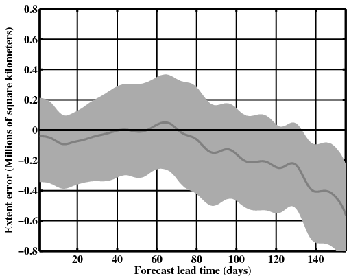
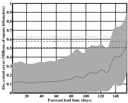
Error vs. lead time Ensemble forecast error (Forecast - observed) in minimum sea ice extent from 1990-2012 as a function of forecast lead time. The median member is denoted by the gray contour while the mean ensemble range is denoted by the light gray shading.		Mean absolute error vs. lead time Mean absolute forecast error in minimum sea ice extent from 1990-2012 as a function of forecast lead time. The median member is denoted by the solid gray contour while the mean ensemble range is enclosed by the gray shading. Light-dashed gray are mean absolute errors for persistence forecasts, while medium-dashed (dark-dashed) are those from first-(second-) order forecasts.

Return to Top